Blackjack: Is It Beatable?
Using Python to See Who Really Wins at Blackjack
With a Master's degree in Economics from McGill University, I currently serve as a Business Analyst in the Revenue Management department at Air Canada. I am eager to learn more about answering tough questions with the help of data analysis, data science, and machine learning. I aspire to become an expert in the field and eventually spend the rest of my days teaching others about math, stats, and data science.
This is my first blog and first Python coding project. I have always been fascinated with casino games, especially Blackjack and Texas Hold'em. The appeal of Texas Hold'em is that if played correctly, it can be beaten. Why? Because your opponents are humans, and humans make mistakes. All I had to do was capitalize on their mistakes to make money in the long term. But Blackjack... Your opponent in Blackjack is not a potentially drunken human staying up too late on a Sunday night. Your opponent is the infamous house, which has supposedly made all the calculations to ensure they will win in the end. No matter how well you play, you will lose in the long run, they say. So, I decided to turn my first coding project into a Blackjack simulator to see if that statement holds true.
Player and Dealer Logic
This section will explain the various choices that were made to make a good attempt at modelling the game of Blackjack. Here are the main important points:
There is an ∞ number of cards (we do not assume a finite number of decks)
The dealer stands on soft 17
A blackjack pays 3 to 2 (unless the player split aces)
The player can double
The player can split equal cards as many times as they'd like
The player can only split aces once, and can only receive one additional card for each ace
The player cannot surrender
The player plays the optimal strategy as shown in this diagram.
The player bets $10 per hand
Simulation Logic
Once we have the logic of the game properly coded, the rest is easy: just press run 100,000 times and manually record the results with a pen and paper. Kidding, of course. We can simply write a little bit of code that will run the game as often as we'd like, while recording the relevant information. But what kind of "relevant information" do we need? We decided to record the following information for every hand that was played:
The sum of the player's first two cards
The sum of all the player's cards (when he is done playing)
The dealer's first card
The sum of all the dealer's cards (when he is done playing)
A boolean where true signifies that the player split his cards during this specific hand, and false signifies that the player did not split his cards
The result (W, L, T)
The money won or lost
The cumulative total money won or lost for a given player
There are three other things that we record for every hand, which can be confusing to explain, so I would like to take the time to elaborate on it here. Here they are:
The simulation number (one game)
The hand number
The meta simulation number (one player)
The simulation number is used to track which iteration of the game we are currently on. For example, let's say the player is playing his 54th game (in other words, his 54th simulation), and is showing an [8,8]. He then decides to take one more card and gets to [8,8,5] for a total of 21. In this case the simulation number would be 54 since this was the 54th simulation for this particular player.
Using the example from above, his hand number would be "0", since this was the first hand he played in the 54th simulation number. Most of the time, the hand number will be "0", since players usually play one hand per game. However, for example, if a player is showing an [8,8] and decides to split his cards, he will then be given 2 hands: [8,3] and [8,5]. Now the [8,3] will be categorized as hand "0", and the [8,5] will be categorized as hand "1".
Finally, the meta simulation number categorizes a given player. As you'll see in the next section, we simulate the game of Blackjack for 100 different players, or, in other words, we have 100 different meta simulations. Let's say player 3 is playing his 55th game and has a [6,5,10], his meta simulation number would be 3, the simulation number would be 55, and the hand number would be 0.
Putting everything together, we get a table that looks like this:

To help read it, the first row shows that for meta simulation number 1 (or player 1), for their first game (first simulation number), and for their first hand (hand 0), their first two cards gave them a total of 16. However, since the dealer was showing a 10, this made them have to "hit" which put them at a total of 26. The final result is a "L (since their sum went above 21) and so the player lost $10, and is currently sitting at -$10 in cumulative earnings.
Results - First Simulation
The first simulation runs the Blackjack game 100 times (100 simulations), records the results, and then does this 100 times (100 meta simulations). Therefore, in total, there are 10,000 simulations being played (with 10,293 hands since the player split a total of 293 times throughout the simulation). The purpose of running the simulation this way is twofold:
To mimic a scenario where a single person plays for 2 hours, which comes down to approximately 100 hands
To simulate observing 100 different people, each playing 100 hands
With each coloured line representing a given player in the figure below, we plot the total profit per player over 100 hands, assuming the player bets $10 per hand:
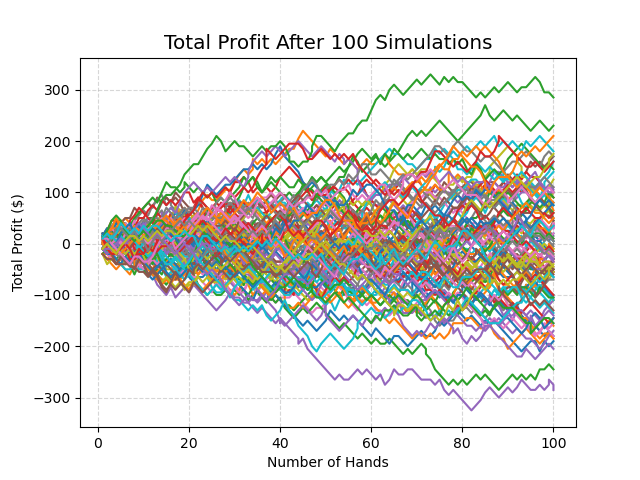
It's interesting to note that the graph doesn't clearly show that the house has an edge. There are a lot of players that are above the $0 line (meaning they secured a profit at the end of the 100 simulations). In fact, in this simulation, we find that out of the 100 players:
45 made a profit , where the average profit was $0.87 per hand
54 made a loss, where the average loss was $0.87 per hand
1 broke even
From the points above, it looks like the player wins 45% of the time. However, this is not the case, since the following shows the amount of individual hands that were won, lost, tied, and the average profit:
| Result | Count | Count (%) | Average Profit |
| Win | 4,449 | 43.22% | $11.84 |
| Loss | 4,895 | 47.56% | -$10.93 |
| Tie | 949 | 9.22% | $0 |
| Total | 10,293 | 100% |
QUESTION: Even though the Player wins at a lower rate than the dealer (43.22% vs 47.56%), the average gain is greater than the average loss ($11.84 vs $10.93). So what's the final result? Are we profitable?
To answer that question, we can plot the distribution of the average profit per hand for every player. Essentially, we look at a given meta simulation i (which represents a player), and we apply the following formula:
$$\frac{\text{(Total Profit or Loss)}_i}{\text{(Total Number of Hands)}_i}$$
So, if a player ended with a profit of $50 after 100 simulations (and 105 hands), then his average profit per hand would be:
$$\frac{$50}{105\text{ hands}} =$0.48\text{/hand}$$
We do this for each player (each meta simulation), and we plot them in the following bar chart:
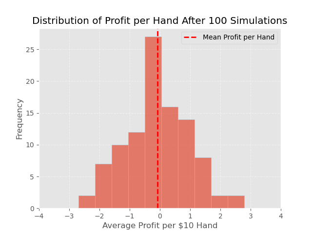
In the plot above, we can see at the most left point, for example, there are roughly 2.5% of players that ended their night with an average loss per hand between -$3 and -2$. However, the red dotted line shows that the average result is a $0.08 loss. We can now answer the question from above.
ANSWER: There are two opposing dynamics: the dealer tends to win more hands, but when the player wins, their winnings are typically larger. The question is, which dynamic has a greater impact overall? Unfortunately, even though the player wins more money during a winning hand, the dealer wins too many hands for the player to remain profitable, which is why we see an average loss of $0.08 as shown in the figure above.
You may be wondering, isn't the sample size of 10,000 total simulations a little small? Maybe this is just a fluke? You may be correct, so let's run this simulation 1,000,000 times.
Results - Second Simulation
In this new simulation, we keep everything the same, except we allow each of the 100 players (meta_simulations) to play 10,000 simulations (instead of 100). This will give us a more accurate depiction of the long-term reality when playing Blackjack.
Let's start by plotting the profit per player across the 10,000 simulations:
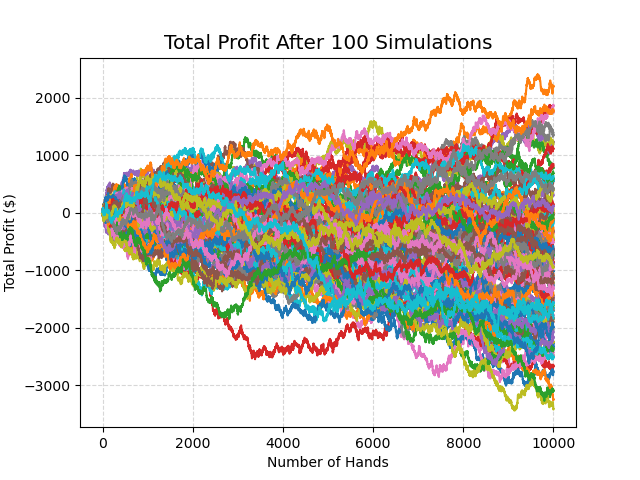
In contrast to the first time we ran this graph, we can more clearly see that there are more cases where a player seems to end in the area below the $0 profit line. In fact, in this simulation, we find that out of the 100 players:
25 made a profit , where the average profit was $0.08 per hand
75 made a loss, where the average loss was $0.13 per hand
This also shows that the more hands a player plays, the less likely it is that they will end the day with a profit. Even though the casino's edge is very small, it adds up quite quickly in the long run.
When we rerun the distribution plot (as shown below), we also see a similar result, where the average loss per hand is steadily at $0.08 per hand.
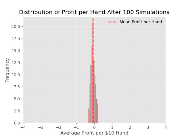
The distribution is significantly narrower compared to the previous simulation. Earlier, the average profit per 10 hands ranged from -$4 to +$4. Now, it fluctuates only between -$0.30 and +$0.20. This reduction in variance is due to the increased number of simulations played (10,000 versus 100). With more simulations played, the results tend to cluster closely around the true average profit per hand.
Consider this analogy: if you flip a coin 10 times, it’s believable to get heads more than 70% of the time (7 or more heads). The probability of this occurrence is roughly 5%. However, if you flip the coin 1,000,000 times, it becomes virtually impossible for heads to appear more than 70% of the time (700,000+ heads). The probability is nearly 0%, as this outcome would be around 400 standard deviations away from the mean. This is an example of the Law of Large Numbers, which was proven by the Swiss mathematician Jakob Bernoulli in 1713, and is widely used in the field of statistics, economics, mathematics, etc.
Conclusion
Our analysis shows that, for this specific type of Blackjack game and assuming the player uses the optimal strategy described here, players will, on average, lose $0.08 per $10 hand. This indicates a house edge of about 0.8%. This edge is highly specific to the conditions outlined at the start of the article. If any of these conditions change—such as a 6 to 5 Blackjack payout, the number of decks used, or restrictions on splitting—the house edge will also change. However, regardless of the Blackjack variation, the house will always have an advantage. The only way to potentially shift the odds in your favor is through card counting, which allows you to adjust your strategy based on the current state of the deck. Implementing a card counting feature in the code could be an interesting next step to explore when it turns the profit in favour of the player.
Thank you for reading the very first blog to be posted on mathieutorchia.com. I am excited to explore more questions and learn new methods on Python along the way. Follow my GitHub here to see the Python code that made this article possible (I am still learning the ins and outs about GitHub so please bear with me - if anyone has any suggestions, I am all ears). And of course, feel free to reach out if you have any questions or comments!


